Writing COMP specifications
A COMP specification consists of a series of modules that introduce either data types or behavioural objects and are interrelated through various data-importation and object-composition operators.
In this tutorial, we discuss only some of the main specification features of COMP.
We introduce them by means of a simple example of a mutual-exclusion protocol.
QLock is a variant of Dijkstra's concept of binary semaphore.
It can be used in systems with multiple execution threads to ensure that distinct processes cannot access a critical resource at the same time.
The basic idea is that, under QLock, every process cycles through three sections: remainder, waiting, and critical.
All processes are initially in the remainder section.
To access the critical section, they must fist announce their intention by switching to the waiting section, which also means entering a waiting queue.
Only the process at the head of the waiting queue is allowed to enter the critical section – after which it can exit to return to the remainder section at any time.
Data types
We begin by specifying the data types used by QLock, namely sections and process identifiers.
For sections, we consider a data module named PC (for Program Counter) with four declarations:
first, of a sort PS (same as the name of the module) that captures the data type of sections;
then, three constants (operations with an empty arity) of sort PC, one for each possible state of a process: rm for the remainder section, wt for the waiting section, and cs for the critical section.
We indicate that these constants are data constructors through the ctor attribute.
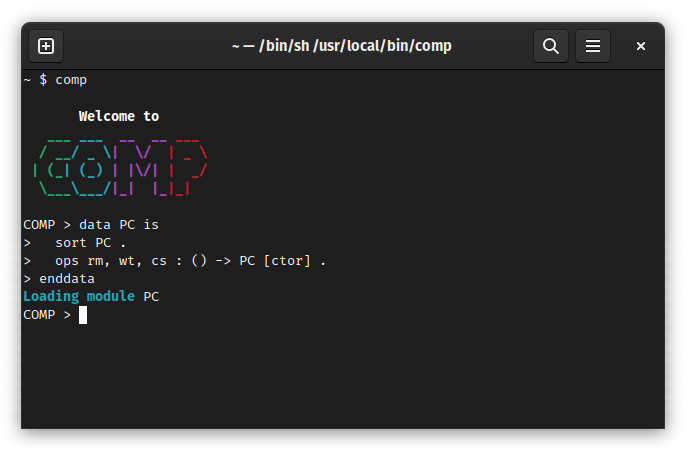
  data PC is
    sort PC .
    ops rm, wt, cs : () -> PC [ctor] .
  enddata
The code can be either typed directly at the COMP prompt or loaded from an external text file.
If all is written correctly and the interpreter accepts the input, you should receive a message of the form
Loading module PC, as in the following image.
Process identifiers are defined by means of natural numbers.
Therefore, before declaring them, we need to load the library Nat.comp, which provides basic support for working with natural numbers.
The file is available (together with Bool.comp, which is used to define relations on natural numbers) in the COMP library of examples.
load Nat.comp
In the module below, we use pid to build process identifiers (pids) from natural numbers, and we form sequences of pids through plain juxtaposition using the mixfix operator __.
Any non-empty (i.e. not nil) sequence is of the form I ... nil, where I is a pid which may be followed by other pids.
For example, the sequence of pids given by the numbers 0, 1, and 2 is written pid(0) pid(s 0) pid(s s 0) nil.
  data PID is
    protecting NAT .

    sort PId .
    op pid : Nat -> PId [ctor] .

    sort PIdSequence .
    op nil : () -> PIdSequence [ctor] .
    op __ : PId PIdSequence -> PIdSequence [ctor] .
  enddata
Next, we define a couple of operations on pids and pid sequences that will be used in the later part of the specification:
just builds a singleton sequence;
add appends a pid at the end of a sequence;
head returns, if possible, the prefix of length one of a sequence, or nil otherwise; and
tail returns the pids after the head of a sequence.
We capture the application of these operations through axioms (in this case, plain equations), which we introduce using the keyword ax.
  data PID/OPS is
    protecting PID .
    vars I, J : PId . var S : PIdSequence .

    op just : PId -> PIdSequence .
    ax just(I) = I nil .

    op add : PId PIdSequence -> PIdSequence .
    ax add(I, nil) = I nil .
    ax add(I, J S) = J add(I, S) .

    ops head, tail : PIdSequence -> PIdSequence .
    ax head(nil) = nil .
    ax head(I S) = I nil .
    ax tail(nil) = nil .
    ax tail(I S) = S .
  enddata
Behavioural objects
We have thus arrived at the objects of the QLock protocol.
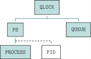
The hierarchical structure of the system is depicted in the diagram below, where PS represents a database of processes (specified by PROCESS) indexed by pids, QUEUE models the waiting queue for accessing the critical section, and QLOCK is the specification of the protocol.
Each solid line denotes a composition of objects.
The first one, from PROCESS, intersecting the dashed line from PID, indicates an indexed composition: PS (the compound object) can be regarded as an arbitrarily large database containing a copy of PROCESS for each pid.
The second one, from PS and QUEUE, indicates a synchronized composition: QLOCK (the compound object in this case) is obtained by putting together the objects PS and QUEUE and by synchronizing them (using additional operations).
Let's start with PROCESS.
A process supports three actions (operations that change the state of the process:
want, to signal the intent to access the critical section;
try, to enter the critical section; and
exit, to leave the critical section.
The actual program counter is given by the observation pc – similarly to actions, observations are defined on process states; however, they do not change those states and return instead some kind of useful data.
We use init to denote the initial state of a process, and axioms to specify how the program counter changes under the effect of the three actions.
Note that, at this stage, since a process has no knowledge of the program counters of other processes, we impose no restriction on the try action (such as checking that the process can really enter the critical section).
That feature is added later on in QLOCK.
  bobj PROCESS is
    protecting PC .
    var S : State .

    op init : () -> State .
    act _>>=`want : State -> State .
    act _>>=`try : State -> State .
    act _>>=`exit : State -> State .

    obs pc : State -> PC .
    ax pc(init) = rm .
    ax pc(S >>= want) = wt .
    ax pc(S >>= try) = cs .
    ax pc(S >>= exit) = rm .
  endbo
To define the process database, we simply use the indexing operator.
We add a constant init to denote the initial state of the database, and an axiom to define the state of every process I (identified by its pid) in the initial state of the database.
So, notice that, in the context of PS, we deal with two kinds of behavioural objects, and thus with two notions of state:
states of processes, denoted PROCESS/State, and states of the process database, denoted State.
  bobj PS is
    indexing PROCESS on PID by PId .
    var I : PId .

    op init : () -> State .
    ax PROCESS/State(I, init) = init .
  endbo
The QUEUE has two defining actions:
enq for adding a new process to the waiting queue; and
deq for removing the top/front process of the waiting queue.
We consider two observations:
one of them, seq, which lists all pids in the queue, is a core observation;
the other, head is derived (i.e., it may be seen as a macro).
In addition, here too we consider an initial state where the queue has no waiting processes.
  bobj QUEUE is
    protecting PID/OPS .
    protecting NAT/PREDECESSOR .
    var Q : State . var I : PId .

    op init : () -> State .
    act _>>=`enq`(_`) : State PId -> State .
    act _>>=`deq : State -> State .
    obs seq : State -> PIdSequence .

    ax seq(init) = nil .
    ax seq(Q >>= enq(I)) = add(I, seq(Q)) .
    ax seq(Q >>= deq) = tail(seq(Q)) .

    obs head : State -> PIdSequence .
    ax head(Q) = head(seq(Q)) .
  endbo
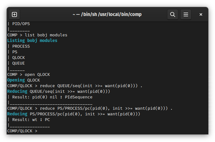
The last object in this tutorial is QLOCK, which synchronizes the process database, PS, with QUEUE.
  bobj QLOCK is
    syncing PS and QUEUE .
    var S : State . var I : PId .

    op init : () -> State .
    ax PS/State(init) = init .
    ax QUEUE/State(init) = init .
Besides the initial state, we also consider three actions: want, try, and exit.
These mirror the actions declared for PROCESS;
however, this time, because they are meant to update the state of the protocol (which includes a database of processes), we need to pass a process id as an additional argument.
For example, for the want action, we write:
act _>>=`want`(_`) : State PId -> State .
We specify how protocol states change under the effect of want in a componentwise fashion.
That is, we axiomatize how each of the two components of QLOCK (PS and QUEUE) is affected by want – and in this way we capture the inner workings of the QLock protocol.
For example, the first of the following four axioms specifies that a process I can enter the waiting queue (in a state S of the protocol) only if its program counter is in the remainder section.
    ax PS/State(S >>= want(I))
     = PS/State(S) >>= want :: PROCESS(I) if PS/PROCESS/pc(I, S) = rm .
    ax PS/State(S >>= want(I))
     = PS/State(S) if not PS/PROCESS/pc(I, S) = rm .
    ax QUEUE/State(S >>= want(I))
     = QUEUE/State(S) >>= enq(I) if PS/PROCESS/pc(I, S) = rm .
    ax QUEUE/State(S >>= want(I))
     = QUEUE/State(S) if not PS/PROCESS/pc(I, S) = rm .
The remaining two actions are defined in a similar manner:
    act _>>=`try`(_`) : State PId -> State .
    ax PS/State(S >>= try(I))
     = PS/State(S) >>= try :: PROCESS(I)
     if PS/PROCESS/pc(I, S) = wt and QUEUE/head(S) = just(I) .
    ax PS/State(S >>= try(I))
     = PS/State(S)
     if not PS/PROCESS/pc(I, S) = wt or not QUEUE/head(S) = just(I) .
    ax QUEUE/State(S >>= try(I))
     = QUEUE/State(S) .

    act _>>=`exit`(_`) : State PId -> State .
    ax PS/State(S >>= exit(I))
     = PS/State(S) >>= exit :: PROCESS(I) if PS/PROCESS/pc(I, S) = cs .
    ax PS/State(S >>= exit(I))
     = PS/State(S) if not PS/PROCESS/pc(I, S) = cs .
    ax QUEUE/State(S >>= exit(I))
     = QUEUE/State(S) >>= deq if PS/PROCESS/pc(I, S) = cs .
    ax QUEUE/State(S >>= exit(I))
     = QUEUE/State(S) if not PS/PROCESS/pc(I, S) = cs .
  endbo
This concludes the specification of the QLock protocol.
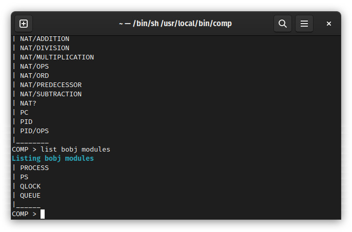
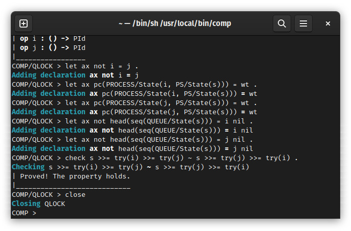
To get a list of all modules that we've loaded so far into the COMP interpreter, we can use the command list modules.
Alternatively, we can use list data modules or list bobj modules to list only data-type or object modules.